3.4. Sums of Series and Complexities of Loops
So far we have seen the complexities of simple straight-line programs, taking the maximum of their asymptotic time demand, using the property of big-O with regard to the maximum. Unfortunately, this approach does not work if the number of steps an algorithm makes depends on the size of the input. In such cases, an algorithm typically features a loop, and the demand of a loop intuitively should be obtained as a sum of demands of its iterations.
Consider, for instance, the following OCaml program that sums up elements of an array:
let sum = ref 0 in
for i = 0 to n - 1 do
    sum := !sum + arr.(i)
done
!sum
Each individual summation has complexity \(O(1)\). Why can’t we obtain the overall complexity to be \(O(1)\) if we just sum them using the rule of maximums (\(\max(O(1), \ldots, O(1)) = O(1)\))?
The problem is similar to summing up a series of numbers in math:
but also
What in fact we need to estimate is how fast does this sum grow, as a function of its upper limit \(n\), which corresponds the number of iterations:
By distributivity of the sums:
In general, such sums are referred as series in mathematics and have the standard notation as follows:
where \(a\) is called the lower limit, and \(b\) is the upper limit. The whole sum is \(0\) if \(a < b\).
3.4.1. Arithmetic series
Arithmetic series are the series of the form \(\sum_{i=a}^{b}i\). Following the example of Gauss, one can notice that
This gives us the formula for arithmetic series:
Somewhat surprisingly, an arithmetic series starting at constant non-1 lower bound has the same complexity:
3.4.2. Geometric series
Geometric series are defined as series of exponents:
Let us notice that
Therefore, for \(a \neq 1\)
3.4.3. Estimating a sum by an integral
Sometimes it is difficult to write an explicit expression for a sum. The following trick helps to estimate sums of values of monotonically growing functions:
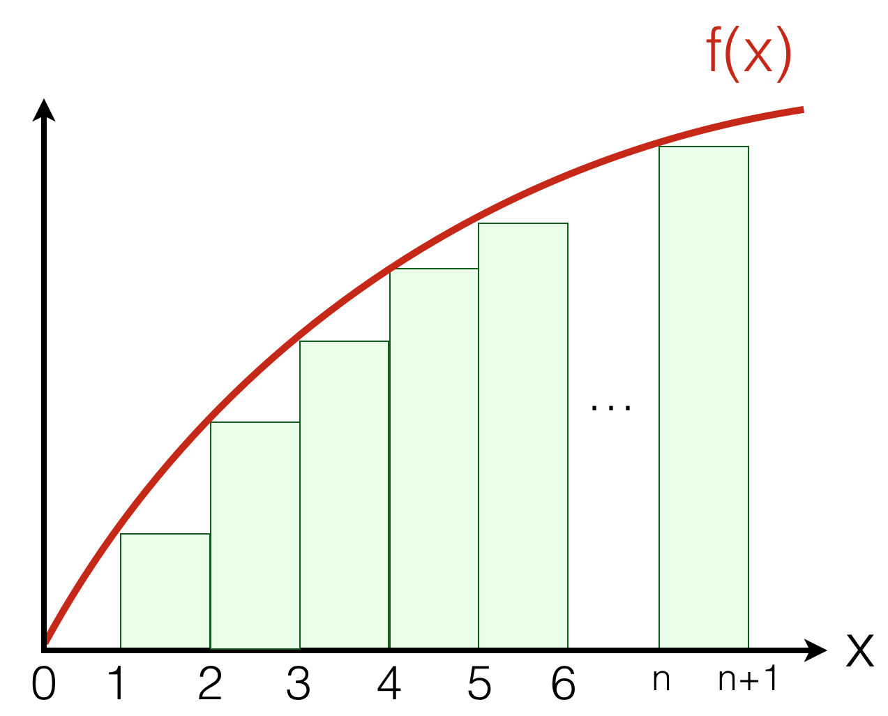
Example: What is the complexity class of \(\sum_{i=1}^{n}i^3\)?
We can obtain it as follows:
3.4.4. Big O and function composition
Let us take \(f_1(n) \in O(g_1(n))\) and \(f_2(n) \in O(g_2(n))\). Assuming \(g_2(n)\) grows monotonically, what would be the tight enough complexity class for \(f_2(f_1(n))\)?
It’s tempting to say that it should be \(g_2(g_2(n))\). However, recalls that by the definition of big O, \(f_1(n) \leq c_1\cdot g_2(n)\) and \(f_2(n) \leq c_2\cdot g_2(n)\) for \(n \geq n_0\) and some constants \(c_1, c_2\) and \(n_0\).
By monotonicity of \(g_2\) we get
Therefore
The implication of this is one should thread function composition with some care. Specifically, it is okay to drop \(c_1\) if \(g_2\) is a polynomial, logarithmic, or their composition, since:
However, this does not work more fast-growing functions \(g_2(n)\), such as an exponent and factorial:
3.4.5. Complexity of algorithms with loops
Let us get back to our program that sums up elements of an array:
let sum = ref 0 in
for i = 0 to n - 1 do
    sum := !sum + arr.(i)
done;
!sum
The first assignment is an atomic command, and so it the last
references, hence they both take \(O(1)\). The bounded
for-iteration executes \(n\) times, each time with a constant
demand of its body, hence it’s complexity is \(O(n)\). To
summarise, the overall complexity of the procedure is \(O(n)\).
Let us now take a look at one of the sorting algorithms that we’ve studies, namely, Insertion Sort:
let insert_sort arr =
  let len = Array.length arr in
  for i = 0 to len - 1 do
    let j = ref i in
    while !j > 0 && arr.(!j) < arr.(!j - 1) do
      swap arr !j (!j - 1);
      j := !j - 1
    done
  done
Assuming that the size of the array is \(n\), the outer loop makes
\(n\) iterations. The inner loop, however, goes in an opposite
direction and starts from \(j\) such that \(0 \leq j < n\)
and, in the worst case, terminates with \(j = 0\). The complexity
of the body of the inner loop is linear (as swap performs three
atomic operations, and the assignment is atomic). Therefore, we can
estimate the complexity of this sorting by the following sum (assuming
\(c\) is a constant accounting for the complexity of the inner
loop body):
With this, we conclude that the complexity of the insertion sort is quadratic in the size of its input, i.e., the length of the array.