2.6. Order Notation
Let us introduce a concise notation for asymptotic behaviour of time demand functions as an input size \(n\) of an algorithm grows infinitely, i.e., \(n \rightarrow \infty\).
2.6.1. Big O-notation
Definition
The positive-valued function \(f(x) \in O(g(x))\) if and only if there is a value \(x_0\) and a constant \(c > 0\), such that for all \(x \geq x_0\), \(f(x) \leq c \cdot g(x)\).
This definition can be illustrated as follows:
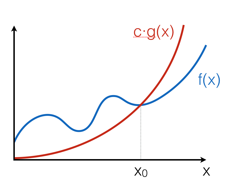
The intuition is that \(f(x)\) grows no faster than \(c \cdot g(x)\) as \(x\) gets larger. Notice that the notation \(O(g(x))\) describes a set of functions, “approximated” by \(g(x)\), modulo constant factors and the starting point.
2.6.2. Properties of Big O-notation
Property 1
\(O(k \cdot f(n)) = O(f(n))\), for any constant \(k\).
Multiplying by \(k\) just means re-adjusting the values of the arbitrary constant factor \(c\) in the definition of big-O. This property ensures machine-independence (i.e., we can forget about constant factors). Since \(\log_{a}n = \log_{a}b \times \log_{b}n\), we don’t need to be specific about the base when saying \(O(\log~n)\).
Property 2 \(f(n) + g(n) \in O(\max(f(n), g(n))\)
Here, \(\max((f(n), g(n))\) is a function that for any n, returns the maximum of \(f(n)\) and \(g(n))\):
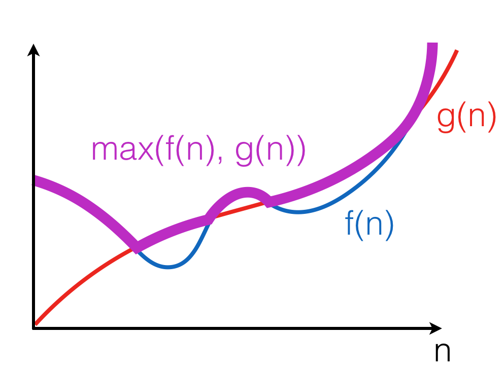
The property follows from the fact that for any \(n, f(n) + g(n) \leq 2 \cdot f(n)\) or \(f(n) + g(n) \leq 2 \cdot g(n)\). Therefore, \(f(n) + g(n) \leq 2 \cdot \max(f(n), g(n))\).
Property 3
\(\max(f(n), g(n)) \in O(f(n) + g(n))\).
This property follows from the fact that for any \(n, \max(f(n), g(n)) \leq f(n)\) or \(\max(f(n), g(n)) \leq g(n)\). Therefore, \(\max(f(n), g(n)) \leq f(n) + g(n)\).
Corollary
\(O(f(n) + g(n)) = O(\max(f(n), g(n))\).
Property 4
If \(f(n) \in O(g(n))\), then \(f(n) + g(n) \in O(g(n))\).
Follows from the fact that there exist \(c, n_0\), such that for any \(n \geq n_0, f(n) \leq c \cdot g(n)\); Therefore, for any \(n \geq n0, f(n) + g(n) \leq (c + 1) \cdot g(n)\). Intuitively, a faster-growing function eventually dominates.
2.6.3. Little o-notation
Definition
The positive-valued function \(f(x) \in o(g(x))\) if and only if for all constants \(\varepsilon > 0\) there exists a value \(x_0\) such that for all \(x \geq x_0, f(x) \leq \varepsilon \cdot g(x)\).
This definition provides a tighter boundary on \(f(x)\): it states that \(g(x)\) grows much faster (i.e., more than a constant factor times faster) than \(f(x)\).
Example
We can show that \(x^2 \in o(x^3)\), as for any \(\varepsilon > 0\) we can take \(x_0(\varepsilon) = \frac{1}{\varepsilon} + 1\), so for all \(x \geq x_0(\varepsilon), \varepsilon \cdot x^3 \geq \varepsilon \cdot (\frac{1}{\varepsilon} + 1) \cdot x^2 > x^2\).
2.6.4. Proofs using O-notation
Standard exercise: show that \(f(x) \in O(g(x))\) (or not) is approached as follows:
- Unfold the definition of O-notation;
- Assuming that the statement is true, try to find a fixed pair of values \(c\) and \(x_0\) from the definition to prove that the inequality holds for any \(x\);
- If such fixed pair cannot be found, as it depends on the value of \(x\), then the universal quantification over \(x\) in the definition doesn’t hold, hence \(f(x) \notin O(g(x))\).
Example 1: Is \(n^2 \in O(n^3)\)?
Assume this holds for some \(c\) and \(n_0\), then:
As this clearly holds for \(n_0 = 2\) and \(c = 1\), we may conclude that \(n^2 \in O(n^3)\).
\(\square\)
Example 2: Is \(n^3 \in O(n^2)\)?
Assume this holds for some \(c\) and \(n_0\), then:
Now, since \(c\) and \(n_0\) are arbitrary, but fixed, we can consider \(n = c + 1 + n_0\) (and so we can do for any \(c\) and \(n_0\)), so we see that the inequality doesn’t hold, hence in this case no fixed \(c\) and \(n_0\) can be found to satisfy it for any \(n\). Therefore \(n^3 \notin O(n^2)\).
\(\square\)
2.6.5. Hierarchy of algorithm complexities

2.6.6. Complexity of sequential composition
Consider the following OCaml program, where a is a value of size n:
let x = f1(a)

in  x + f2(a)
Assuming the complexity of f1 is \(f(n)\) and the complexity of f2 is \(g(n)\), executing both of them sequentially leads to summing up their complexity, which is over-approximated by \(O(\max(f(n), g(n))\). This process of “collapsing” big O’s can be repeated for a finite number of steps, when it does not depend on the input size.
2.6.7. Exercise 6
Assume that each of the expressions below gives the time demand \(T(n)\) of an algorithm for solving a problem of size \(n\). Specify the complexity of each algorithm using big \(O\)-notation.
- \(500n + 100n^{1.5} + 50n \log_{10}n\)
- \(n \log_3 n + n \log_2 n\)
- \(n^2 \log_2 n + n (\log_2 n)^2\)
- \(0.5 n + 6n ^{1.5} + 2.5 \cdot n ^{1.75}\)
2.6.8. Exercise 7
The following statements provide some “properties” of the big O-notation for the functions \(f(n)\), \(g(n)\) etc. State whether each statement is TRUE or FALSE. If it is true, provide a proof sketch using the properties of the O-notation. If it is false, provide a counter-example, and if you a way to fix it (e.g., by changing the boundary on the right), provide a “correct” formulation a proof sketch while it holds.
- \(5 n + 10 n^2 + 100 n^3 \in O(n^4)\)
- \(5n + 10n^2 + 100 n^3 \in O(n^2 \log n)\)
- Rule of products: \(g_1 (n) \in O(f_1(n))\) and \(g_2 (n) \in O(f_2(n))\), then \(g_1 (n) \cdot g_2 (n) \in O(f_1(n) \cdot f_2(n))\).
- Prove that \(T_n = c_0 + c_1 n + c_2 n^2 + c_3 n^3 \in O(n^3)\) using the formal definition of the big \(O\) notation.
2.6.9. Exercise 8
One of the two software packages, A or B, should be chosen to process data collections, containing each up to \(10^{12}\) records. Average processing time of the package A is \(T_A(n) = 0.1 \cdot n \cdot \log_2 n\) nanoseconds and the average processing time of the package B is \(T_B(n) = 5 \cdot n\) nanoseconds. Which algorithm has better performance in the big \(O\) sense? Work out exact conditions when these packages outperform each other.
2.6.10. Exercise 9
Algorithms A and B spend exactly \(T_A(n) = c_A \cdot n \cdot \log_2 n\) and \(T_B(n) = c_B \cdot n^2\) nanoseconds, respectively, for a problem of size \(n\). Find the best algorithm for processing \(n = 2^{20}\) data items if the algorithm A spends 10 nanoseconds to process 1024 items, while the algorithm B spends only 1 nanosecond to process 1024 items.